Building a model¶

In this section we will look at pratical example of how we can build a regression model to see how whether membrane resistance, spike threshold and resting membrane potential contribute to rheobase. Often we just want to test whether our measure is different between genotype, treatment, sex, etc. However, we can actually build a more biological plausible model that also gets into some simple causal analysis. This analysis will also cover several techniques such as model comparison, residual analysis and intepretation of regression coefficients. One thing to note is that rheobase is specifically excludes the effects of capacitance since we measure it with an infinitely long current injection. Additionally, this dataset seems to have bimodal capacitance which will throw off the whole regression equation so we are leaving out of the model but showing the data here. Another benefit of building a model with this dataset is that it will touch on some core regression modeling methodology, namely non-linear relationships and some mediation analysis.

Setting the baseline¶

First we are going to see how well predicted rheobase matches up to the actual rheobase. We can use the simple equation $\Delta V=IR_m$ for the relationship between resistance and rheobase. To get $\Delta V$ we will subtract the resting membrane potential from the spike threshold. To get $I$ we will divide $\Delta V$ by $R_m$. We will regress the predicted rheobase against the actual rheobase using a simple linear regression. Then we will analyze the regression output.

Load and prepare the data¶

The dataset being used for this chapter is the same data used for the MSN data in other chapters. I and others recorded D1-tdTom+ and D1-tdTom- cells from adult mice (~P90). A couple notes on how the data was analyzed. Membrane resistance was measured using the currents injections from -150 to 150 and is the slope coefficient of the regression current ~ delta_v. A slow current was injected to keep the cells close to -70 mV. The spike threshold was measured using the peak of the third derivative. Capacitance (Cm) was measured on break-in using a test pulse. To prepare our dataset we will need to rename our columns so we can use the statsmodels formula API. This means we need to remove spaces, parenthesis, brackets, etc. for the column names.

Run the regression¶

Plot the resulting fit and the points.

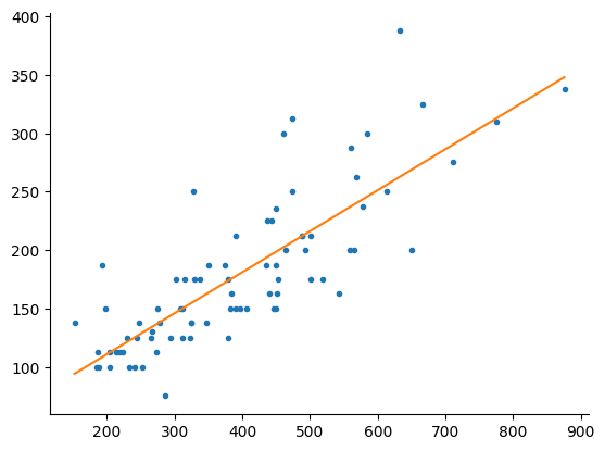
The fit looks goods, but how good is it? Notice how the predicted rheobase seems about 2x larger than the actual rheobase. We can look at the actual model to get more information about this relationship.

Analyze the regression¶

Some things to note about the model summary. Our slope coefficent, synth_rheo is 0.3509 which means if we compare one cell with a rheobase of say 100 and one with a rheobase of 101 the difference in actual rheobase between the two cells would be 0.3509. This means our input needs to be multiplied by 0.3509 to get to the actual rheobase. This is pretty close to the estimate of the predicted rheobase being 2x larger than the actual rheobase. Why is the slope not close to one? It might depend on how we measure membrane resistance. For this data set the cell was held at -70 mV by injecting a slow (DC) current. I regressed the delta v against the current injection amplitude only for acquisition with 150 pA of the 0 pA current injection. We have different sets of ion channels that are active at current injections. Ih channels open below -40 mV, Na+ channels start to open with depolarizing current injections, K+ leak channels are probably more important around the resting membrane potential just to name a few. What if we break down the predicted rheobase into its components? Lastly we should look at the confidence intervals to get an idea of how good our estimate is. Even though p < 0.05 this does not mean our estimate is precise it just means the confidence intrevals do not contain zero. A rule of thumb is if you are running and OLS or some variant such as weighted or robust regression, you do not log transform your outcome variable and your confidence intervals do not contain zero the take the ratio of the intervals where the absolute value of the larger interval is on top: abs(large)/abs(small). A rule of thumb is if this interval is > 3 then we have a weak effect. If you have log transformed your outcome then you need to exponentiate your coefficient and confidence intervals first. The exponentiated confiden. So for regression 0.408/0.294=1.388. So we can say that we are fairly confident in our slope measurement regardless of the p-value. If your confidence intervals contain zero then you need to decide on something called a region of pratical equivalence using two one-sided tests (TOST). Or you can decide on an effect size that is practical. Lastly we can look at Adj. R-squared to see how much variance is explained by our model. Adj. R-squared is like R-squared except that it is adjusted for sample size and number of coefficients. Adj. R-squared and R-squared actually converge when the estimated relationship is strong or you have a large sample size. One problem with Adj. R-squared is it is supposed to show us how variance is explained by our model but, it can be negative. This does not really matter because a R-squared close to zero means we explain vary little about the outcome variable with our model. Adj. R-squared at 0.654 is pretty good. That means 64% of our outcome is explained by our predictors. Later we will compare the Adj. R-squared of different models to get a sense of how big 0.654 really is.

Begining to breakdown the model¶

First let’s look at how the different components may be related.

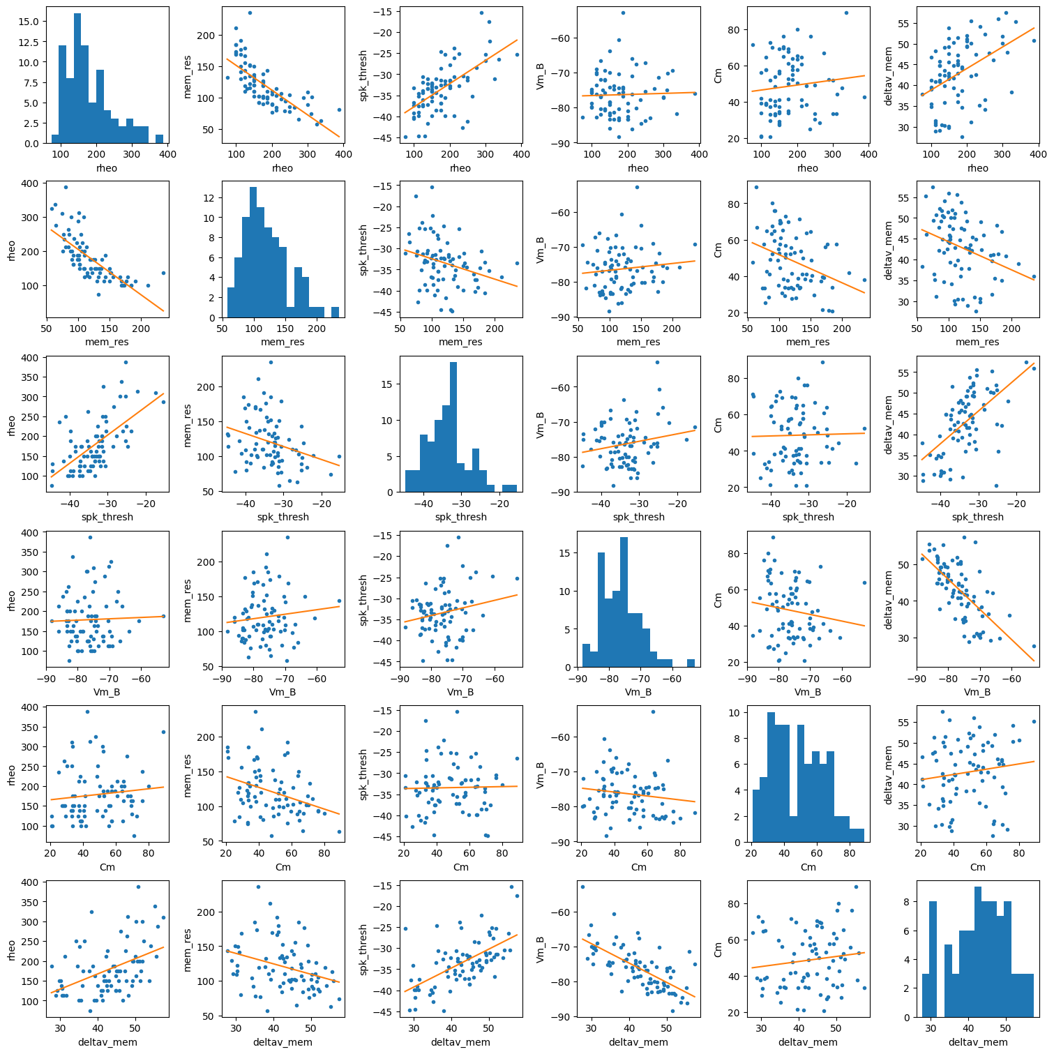
Probably the two biggest things that stand out are that membrane resistance and spike threshold seem to have some relationship with rheobase. The relationship between rheobase and membrane resistance is nonlinear. This makes sense since rheobase and membrane resistance are inversely proportional. Spike threshold is also negatively correlated with membrane resistance where as resting membrane potential is positively correlated. While there seem to be some linear relations between other variables the variance around the simple regression line is quite a lot. When we build a regression model with more predictors we want to avoid collinear features since this will impair the regression fit. Also if we look at the histogram distributions we can see that most variables are left skewed (tail to the right). This could be because of how we measure the membrane resistance. Since I injected a slow current to keep the cells as -70 mV this could change the types of ion channels that are being sampled.

Breaking down predicted rheobase¶

We know that to our predicted rheobase comes from the equation $I = \Delta V/R_m$. This equation is nonlinear so to make is linear we can use a log transform $log(I) = log(\Delta V) - log(R_m)$. Now we have an equation where we can find the relative contribution of $\Delta V$ and $R_m$. However, we cannot easily decompose $\Delta V=Vt-Vm$. To decompose that we know that $V_t$ and $V_m$ are going to explain 100% of the variance in $\Delta V$ so we can just measure the variance by getting the joint variance $\text{Var}(aX + bY) = a^2\text{Var}(X) + b^2\text{Var}(Y) + 2ab\text{Cov}(X,Y)$. For $\Delta V$ we can ignore $a$ and $b$ since they will be 1. You can test this by running a regression delta_v ~ vm + vt and your coefficients will be 1 and -1 since 100% of the variance is explained. Then we can get the contributions for $V_t$ and $V_m$ with the following equations ${V_t} = \frac{\text{Var}(V_t) - \text{Cov}(V_t, V_m)}{\text{Var}(\Delta V)}$ and ${V_m} = \frac{\text{Var}(V_m) - \text{Cov}(V_t, V_m)}{\text{Var}(\Delta V)}$

So we have about equal contribution of $V_m$ and $V_t$ to the variance of $\Delta V$. Next let us see how much $\Delta V$ and $R_m$ predict rheobase.

With this model we can see that most of rheobase is predicted by membrane resistance and less by delta V. Next we can run some simple models where we see how the coefficient changes.

We see that for both membrane resistance and delta V we get larger coefficients. This suggests that there is some correlation between those two variables. We can check that.

There is some correlation but a not a lot. Why can’t we perfectly predict rheobase with delta V and membrane resistance? There are several factors. One is likely due to how we measure membrane resistance using small current injections near the resting membrane potential. Both those variables are capturing the same information. Additionally, resting membrane potential is likely a noisy parameter. So when combined with the spike threshold to calculate delta V we get a less precise parameter. We can also see that the adjusted R2 is much higher for the membrane resistance model than the delta V model. We find that membrane resistance is a primary factor in rheobase. Delta V is probably a minor factor because membrane voltage dynamics are nonlinear.