Current clamp: Part 1 - Patch Clamp Handbook

In part 1 of the current clamp section we will cover how to extract data from current clamp acquisitions. We will focus on pulse injections and not cover ramp injections.

Import the Python packages.

import json
import urllib
from collections import defaultdict

import matplotlib.pyplot as plt
import numpy as np
import pandas as pd
from bokeh.io import output_notebook, show
from bokeh.layouts import column, gridplot, row
from bokeh.models import ColumnDataSource, CustomJS, Slider, Spinner
from bokeh.plotting import figure
from scipy import optimize, signal, stats

output_notebook()

Next we are going to load the data. All the data is stored on json files. While this file type is not the most practical for storing electrophysiological data, it is the very convenient since it does not require any third party python packages.

temp_path = "https://cdn.jsdelivr.net/gh/LarsHenrikNelson/PatchClampHandbook/data/current_clamp/"
exp_dict = {}
for index in range(1, 69):
    url = urllib.request.urlopen(temp_path + f"{index}.json")
    temp = json.load(url)
    temp["array"] = np.array(temp["array"])
    exp_dict[index] = temp
x_array = np.arange(len(exp_dict[1]["array"])) / 10

The first thing to do is look through your data just to see what it looks like. For reference the data in this tutorial is from a layer 5 cell in the ACC of a P16 mouse.

The recorded data is usually in mV, as is the case for this data.
There is a short baseline of about 300 ms before the current injection starts.
There are current injections that make the voltage go negative and ones that the cell goes positive.
There is a point where the positive current injections make the cell spike.
The current injection is finite but also not short enough that only one spike is ever evoked. This is important for calculating the FI curve
There are 4 cycles where the pulse amplitude start at -100 pA and is increased in 25 pA steps until 300 pA is reached.

# Initial data
source = ColumnDataSource(data={"x": np.arange(20000) / 10, "y": exp_dict[1]["array"]})

# Create a plot
plot = figure(
    x_axis_label="Time (ms)", y_axis_label="Voltage (mV)", width=400, height=300
)
plot.line("x", "y", source=source, line_color="black")
spinner = Spinner(title="Acquisition", low=1, high=68, step=1, value=1, width=80)

# JavaScript callback to fetch JSON data and update plot
callback = CustomJS(
    args=dict(source=source, spinner=spinner),
    code="""
    let val = spinner.value
    let URL = `https://cdn.jsdelivr.net/gh/LarsHenrikNelson/PatchClampHandbook/data/current_clamp/${val}.json`
    fetch(URL)
    .then(response => response.json())
    .then(data => {
        source.data.y = data["array"];
        source.change.emit();
    })
    .catch(error => console.error('Error fetching data:', error));
""",
)

# Add a button to trigger the callback
spinner.js_on_change("value", callback)

# Layout and show
layout = column(spinner, plot)
show(layout)

First, we will define some important features of the acquisition so that we can reuse the settings throughout the analysis. It is important to note the all the parameters are going to be in samples. The current files were recorded at 10000 Hz so we are multiply the time by 10.

baseline_start = 0
baseline_end = 3000
pulse_start = 3000
pulse_end = 10000

Measuring delta V and getting the IV curve¶

The first concept we are going to cover is delta V and analyzing the IV (current-voltage curve). Delta V is simply the change in voltage due to the current injection. The IV curve is used to calculate the membrane resistance. Remember that voltage difference = current * resistance ( $\Delta V=IR$ ). This can be calculated by finding the baseline voltage of the acquisition and subtracting voltage during the pulse. There are some things consider when calculating the voltage during the current injection. There can be changes in voltage due channels that temporarily open such as due to Ih channels. To avoid the contribution of these channels I recommend get the mean voltage of the current injection in the last 50%, or even 30%, of the current injection.

acq = exp_dict[1]["array"]
x = np.arange(20000) / 10

# We define the baseline as the mean of the acquisiton from 0 to 300 ms
baseline_v = np.mean(acq[baseline_start:baseline_end])

# We define the pulse voltage as the mean of the acquisition for the last 50% of the current injection
p50 = ((pulse_end - pulse_start) // 2) + pulse_start
injection_v = np.mean(acq[p50:pulse_end])
delta_v = injection_v - baseline_v

fig, ax = plt.subplots()
_ = ax.set_xlabel("Time (ms)")
_ = ax.set_ylabel("Voltage (mV)")
_ = ax.plot(x, acq, color="black", label="Acquisition")
_ = ax.plot(
    x[baseline_start:baseline_end],
    acq[baseline_start:baseline_end],
    color="#37f2fc",
    label="Baseline",
)
_ = ax.plot(
    np.arange(p50, pulse_end) / 10,
    acq[p50:pulse_end],
    color="#fcba37",
    label="Pulse",
)
_ = ax.plot(
    [p50 / 10, p50 / 10],
    [baseline_v, injection_v],
    color="#fc37fc",
    label="Delta V",
)
_ = ax.legend()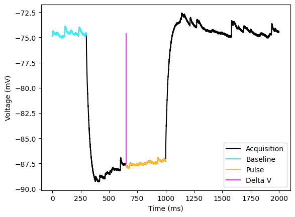

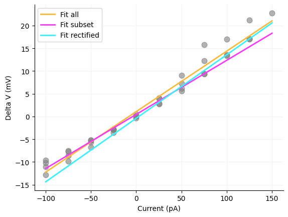
Next we will need to measure the delta V for all pulses except those with spikes. The reason that we do not measure the delta V for acquisitions with spikes is that spiking activity is a seperate state compared to non-spiking. So we will simply exclude acquisitions with spikes. We will do this by ignoring acquisitions with voltages greater than -20 mV. We will also need the pulse amplitude of each acquisition which is located in the file.

You will notice there is a linear relationship between current and voltage. To get the membrane resistance from these data we just have to run a linear regression between the current and delta V. There are a couple ways that you can run the linear regression. One is you can take all delta Vs, you can take just a subset or you can rectify or take the absolute value of the delta Vs before running the regression. We will do all three since it is easy to do in Python. One really important thing to note is the units of the regressors. current is in pA and delta V is in mV and we need to get to MOhms. To do this we multiply the slope by 1000 to get MOhm. If you run the code below you see that the answers are fairly close. One reason to choose the subset version is that you may change the membrane resistance as the cell gets close to spiking even if it does not spike. However, all three calculations are valid.

p50 = ((pulse_end - pulse_start) // 2) + pulse_start
delta_v = []
current_amplitude = []
for acq_num, acq in exp_dict.items():
    voltages = acq["array"]
    baseline_v = np.mean(voltages[baseline_start:baseline_end])
    acq["baseline_v"] = baseline_v
    if np.max(voltages) < -20:
        current_amplitude.append(acq["pulse_amp"])
        injection_v = np.mean(voltages[p50:pulse_end])
        delta_v.append(injection_v - baseline_v)
        acq["delta_v"] = injection_v - baseline_v
    else:
        acq["delta_v"] = np.nan

mem_res_all = stats.linregress(current_amplitude, delta_v)
subset = np.where(np.array(current_amplitude) <= 50)[0]
mem_res_subset = stats.linregress(
    np.array(current_amplitude)[subset], np.array(delta_v)[subset]
)
mem_res_rectified = stats.linregress(np.abs(current_amplitude), np.abs(delta_v))

# \n is just added to print on separate lines
print(
    f"All values: {mem_res_all.slope * 1000}",
    f"Subset: {mem_res_subset.slope * 1000}",
    f"Rectified: {mem_res_rectified.slope * 1000}",
    sep="\n",
)
x_fit = np.linspace(min(current_amplitude), max(current_amplitude), num=50)
fig, ax = plt.subplots()
_ = ax.grid(which="both", color="0.95")
ax.set_axisbelow(True)
_ = ax.set_xlabel("Current (pA)")
_ = ax.set_ylabel("Delta V (mV)")
_ = ax.scatter(
    current_amplitude, delta_v, facecolor="grey", edgecolor="grey", s=60, alpha=0.6
)
_ = ax.plot(
    x_fit,
    mem_res_all.intercept + x_fit * mem_res_all.slope,
    label="Fit all",
    color="#fcba37",
    linewidth=2,
)
_ = ax.plot(
    x_fit,
    mem_res_subset.intercept + x_fit * mem_res_subset.slope,
    label="Fit subset",
    color="#fc37fc",
    linewidth=2,
)
_ = ax.plot(
    x_fit,
    mem_res_rectified.intercept + x_fit * mem_res_rectified.slope,
    label="Fit rectified",
    color="#37f2fc",
    linewidth=2,
)
_ = ax.legend()
ax.spines["right"].set_visible(False)
ax.spines["top"].set_visible(False)

All values: 133.09736486992492
Subset: 119.0104625490823
Rectified: 139.79142592501782

Ih voltage sag¶

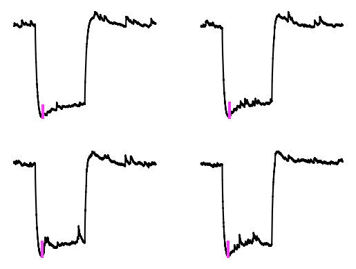
Hyperpolarization-activated cyclic nucleotide–gated (HCN) channels are typically responsible for the voltage sag in a current clamp acquisitions. Voltage sag is when the voltage drop is initially larger at the beginning of the current injection than at the end. Many cell types have Ih voltage sag such as dopaminergic cells and layer 5 pyramidal neurons. Measuring voltage sag is fairly straightforward. You just measure the voltage difference between the peak sag and and the voltage in the second half of the current injection similar to measuring delta V. The main way I have seen voltage sag reported is by measuring the sag on the most negative current injection. You could also technically run an IV curve for the voltage sag. To truly determine whether the voltage sag is due to HCN channels you would need to do a flow-in experiment with the drug ZD7288. If you want to run the IV curve I challenge you to modify the IV code above to get the resistance of the channels contributing to the voltage sag.

p50 = ((pulse_end - pulse_start) // 2) + pulse_start
delta_v = []
current_amplitude = []
sag_loc = []
acqs = []
for acq_num, acq in exp_dict.items():
    voltages = acq["array"]
    if acq["pulse_amp"] == -100:
        acqs.append(voltages)
        current_amplitude.append(acq["pulse_amp"])
        sag_v = np.min(voltages[pulse_start:p50])
        sag_loc.append(np.argmin(voltages[pulse_start:p50]) + pulse_start)
        injection_v = np.mean(voltages[p50:pulse_end])
        delta_v.append(sag_v - injection_v)
        acq["Sag (mV)"] = sag_v
        acq["Sag (ms)"] = np.argmin(voltages[pulse_start:p50]) + pulse_start
    else:
        acq["Sag (mV)"] = np.nan
        acq["Sag (ms)"] = np.nan
print(f"Voltage sag: {np.mean(delta_v):.3f} mV")

Voltage sag: -1.916 mV

Let’s confirm that the voltage sag was correctly measured. Note that when we collected the sag location above we collected the sample number so that needs to be converted to time in ms by dividing by 10.

plots = []
fig, ax = plt.subplots(nrows=2, ncols=2)
for sloc, dv, vs, a in zip(sag_loc, delta_v, acqs, ax.flat):
    a.plot(x_array, vs, color="black")
    a.plot(
        [sloc / 10, sloc / 10],
        [vs[sloc], vs[sloc] - dv],
        color="#fc37fc",
        linewidth=3,
    )
    a.axis("off")

Rheobase¶

Rheobase is the minimum current required to get a cell to spike. This measure is directly related to membrane resistance through the equation: V=IR. When resistence increases, the current need to achieve the same delta V decreases. This means that a cell will higher membrane resistance will likely need less synaptic to be able to spike. There are a couple ways you can find rheobase. Find the minimum current needed to get the cell to spike out of all 4 cycles. I do not recommend this since there is variability between cycles and the variability could be affected by a treatment or other factors. Find the minimum current needed to get the cell to spike for each cycle and average the result. This is the method I recommend. The way I find rheobase below depends on the acquisitions being assigned to a cycle (1 to inf) which ClampSuite automatically. This may not be the case for your data. There are other ways to find rheobase

rheobase = []
rheobase_acq = []
exp_dict[1]["rheobase"] = False
for index in range(2, len(exp_dict) + 1):
    exp_dict[index]["rheobase"] = False
    if (np.max(exp_dict[index]["array"]) > 30) & (
        np.max(exp_dict[index - 1]["array"]) < 30
    ):
        rheobase.append(exp_dict[index]["pulse_amp"])
        rheobase_acq.append(index)
        exp_dict[index]["rheobase"] = True
print(f"Rheobase: {np.mean(rheobase)} pA")

Rheobase: 143.75 pA

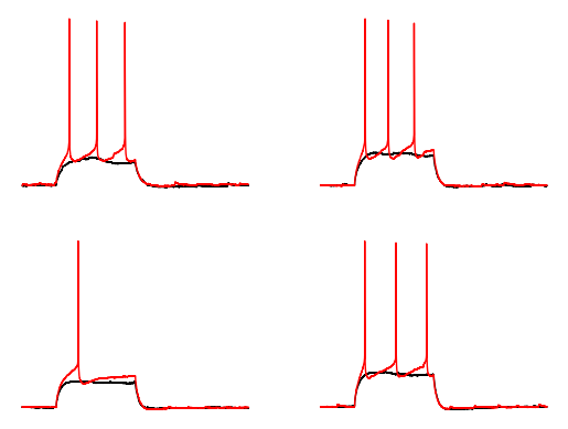
Let’s confirm that we have the right rheobase values by plotting the rheobase acquistion in red and the previous acquisition in black.

plots = []
fig, axes = plt.subplots(nrows=2, ncols=2)
for acq, ax in zip(rheobase_acq, axes.flat):
    ax.plot(x_array, exp_dict[acq - 1]["array"], color="black", linewidth=1)
    ax.plot(x_array, exp_dict[acq]["array"], color="red", linewidth=1)
    ax.axis("off")

Spike frequency¶

Spike frequency is used to create the FI curve. The FI curve relates several pieces of information such as rheobase, gain and maximum firing rate. The firing rate is calculated as the number of spikes that occur during the current injection or you can derive the firing rate from the inter-event (spike) interval (IEI or ISI). The IEI/ISI requires that you have at least two spikes in the acquisition. IEI/ISI is also useful because you can derive the firing rate variability within an acquisition. Three important features you can get from the FI curve that you will need to curve fit to get.

Slope/gain: The input gain of a cell
Maximum firing rate: The response gain of a cell
Current offset
The voltage offset: This is usually close to zero

If you want to learn more about gain I would recommend looking at Ferguson and Cardin, 2020 Ferguson & Cardin, 2020. The Sigmoid curve and gain are explained in-depth below. If you are using the Jupyter Notebook version of the tutorial there is an interactive widget that allows you change the input and output gain of a the Sigmoic curve which can help understand how the different parameters change the curve.

Sigmoid fit the FI curve to get the gain and max firing rate¶

Many papers will just analyze their FI data using a repeated measures ANOVA. However, this method only tells whether or not the FI curves are different and where they are different. To get a better idea of why the curves are different you really need to fit a sigmoid function data for each cell. This will get you the gain of a cell or the slope of the FI curve as well as the estimated maximum firing rate and the current offset. This is a simple example of how to do this in Python.

Understanding gain¶

Below is an example of how changes in gain would work. Note that to get a input gain difference without a rheobase difference the midpoint current has to be changed. That means to test whether there is a gain difference you will like nead to run a multivariate regression or ANOVA because these two factors are not independent.

def sigmoid(x, max_value, midpoint, slope, offset):
    return 1 / (1 + np.exp((x - midpoint) / slope)) * max_value + offset


x = np.linspace(0, 400)
fig, ax = plt.subplots(ncols=3, figsize=(10,4))
ax[0].set_title("Input gain difference")
ax[0].plot(x, sigmoid(x, 17, 200, -40, 0))
ax[0].plot(x, sigmoid(x, 17, 170, -30, 0), color="orange")
ax[1].set_title("Response gain difference")
ax[1].plot(x, sigmoid(x, 20, 200, -40, 0))
ax[1].plot(x, sigmoid(x, 17, 200, -40, 0), color="orange")
ax[2].set_title("Rheobase difference")
ax[2].plot(x, sigmoid(x, 17, 200, -40, 0))
ax[2].plot(x, sigmoid(x, 17, 150, -40, 0), color="orange")
for i in ax:
    i.spines["right"].set_visible(False)
    i.spines["top"].set_visible(False)
    i.grid(axis='both', color='0.95')

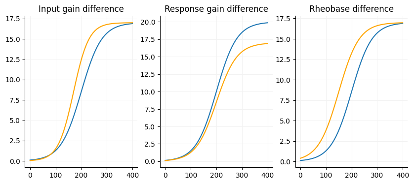
Below is a simple interactive plot where you can play arount with the slope, max value and the midpoint of two sigmoid curves to get an idea of how each of the factors.

def sigmoid(x, max_value, midpoint, slope, offset):
    return 1 / (1 + np.exp((x - midpoint) / slope)) * max_value + offset


x = np.linspace(0, 400)
y1 = sigmoid(x, 16.0, 200.0, -40.0, 0)
y2 = sigmoid(x, 16.0, 200.0, -40.0, 0)

source1 = ColumnDataSource({"x": np.linspace(0, 400), "y1": y1, "y2": y2})
source2 = ColumnDataSource(
    {"x": np.linspace(0, 400, num=49), "y1": np.diff(y1), "y2": np.diff(y2)}
)

plot1 = figure(width=300, height=300)
plot1.line("x", "y1", source=source1, line_width=3, line_alpha=0.6)
plot1.line("x", "y2", source=source1, line_width=3, line_alpha=0.6, line_color="orange")
plot2 = figure(width=300, height=300)
plot2.line("x", "y1", source=source2, line_width=3, line_alpha=0.6)
plot2.line("x", "y2", source=source2, line_width=3, line_alpha=0.6, line_color="orange")

max_val_1 = Slider(value=16.0, start=10.0, end=30.0, step=1.0, title="Response gain 1")
slope_1 = Slider(value=-40, end=-5.0, start=-60.0, step=1.0, title="Input gain 1")
midpoint_1 = Slider(
    value=200.0, start=25.0, end=400.0, step=1.0, title="Current offset 1"
)

callback = CustomJS(
    args=dict(
        source1=source1,
        source2=source2,
        max_val_1=max_val_1,
        slope_1=slope_1,
        midpoint_1=midpoint_1,
    ),
    code="""
    const data = source1.data;
    const x_array = data['x'];
    const y1 = x_array.map((x) => {
        return 1 / (1 + Math.exp((x - midpoint_1.value) / slope_1.value)) * max_val_1.value
    })
    source1.data['y1'] = y1
    const y1_diff = y1.slice(1).map((value, index) => value - y1[index])
    source2.data['y1'] = y1_diff
    source1.change.emit();
    source2.change.emit();
""",
)

max_val_1.js_on_change("value", callback)
slope_1.js_on_change("value", callback)
midpoint_1.js_on_change("value", callback)

show(
    column(
        column(max_val_1, slope_1, midpoint_1),
        gridplot([[plot1, plot2]]),
    )
)

Fit the data to a sigmoid curve¶

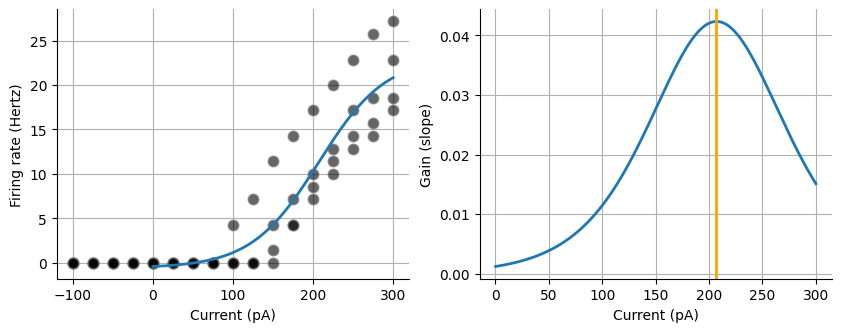
First let’s look at the FI data that we extracted from the acquisitions. We are going to curve fit the FI curve. We will use Scipy’s curve_fit. This function needs a function passed to it, in this case it is the sigmoid function as well as an array for the x values and y values. There are many other factors that you could pass, such as bounding factors but are not needed in this case. Lastly you can fit the entire array of current values, however neurons will only spike when there is a net positive current injection. We can truncate our arrays of current and hertz so that only the pairs that have a current >= 0 are kept. You can fit the sigmoid curve to whole set of data and it will likely fit well.

spike_analysis = {"acqs": [], "hertz": [], "current": [], "peaks": [], "voltages": []}
time = (pulse_end - pulse_start) / 10000

for acq_num, acq in exp_dict.items():
    voltages = np.array(acq["array"])
    peaks, _ = signal.find_peaks(
        voltages[pulse_start:pulse_end],
        height=10,
        prominence=10,
    )
    peaks += pulse_start
    spike_analysis = {}
    spike_analysis["hertz"] = len(peaks) / time
    spike_analysis["current"] = acq["pulse_amp"]
    spike_analysis["peaks"] = peaks
    spike_analysis["voltages"] = voltages[peaks]
    acq.update(spike_analysis)

current = np.array([i["current"] for i in exp_dict.values()])
hertz = np.array([i["hertz"] for i in exp_dict.values()])

indexes = np.where(current >= 0)[0]
lb = [-np.inf, -np.inf, 1e-6, 0]
ub = [np.inf, np.inf, np.inf, np.inf]
p0 = [np.max(hertz[indexes]), np.mean(current[indexes]), 30, 0]
p, _ = optimize.curve_fit(sigmoid, current[indexes], hertz[indexes])
fit_x = np.linspace(0, max(current), 1000)
fit_y = sigmoid(fit_x, p[0], p[1], p[2], p[3])

fig, ax = plt.subplots(ncols=2, figsize=(10,3.5))
ax[0].set_xlabel("Current (pA)")
ax[0].set_ylabel("Firing rate (Hertz)")
ax[0].scatter(
    current,
    hertz,
    color="black",
    edgecolor="grey",
    s=60,
    alpha=0.6,
)
ax[0].plot(fit_x, fit_y, linewidth=2)

diff = np.diff(fit_y)
max_gain_index = diff.argmax()
max_gain = diff[max_gain_index]
max_current = fit_x[max_gain_index]

ax[1].set_xlabel("Current (pA)")
ax[1].set_ylabel("Gain (slope)")

ax[1].plot(fit_x[1:], diff, linewidth=2)
ax[1].axvline(
    x=max_current, color="orange", linewidth=2
)
for i in ax:
    i.spines["right"].set_visible(False)
    i.spines["top"].set_visible(False)
    i.grid(which="both")
    i.set_axisbelow(True)

print(
    f"Slope (gain): {p[2]}",
    f"Max value: {p[0]}",
    f"Midpoint: {p[1]}",
    f"Max gain: {max_gain}",
    sep="\n",
)

Slope (gain): 42.097933962917814
Max value: -23.74029449005258
Midpoint: 206.89907926786566
Max gain: 0.04233693298645491

Spike adaptation index¶

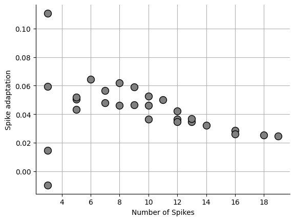
Spike adaptation is a way to quantify whether IEI is stable or not. Some cells such as fast spiking interneurons have an extremely stable IEI that changes very little as spike frequency increases. Other cells types such as layer 5 pyramidal cells have an IEI that increase as spike frequency increases. There are many ways to calculate the spike adaptation and we will cover a few of them here.

Allen institute method¶

This method is ideal if you want to know if your IEIs are increasing or decreasing since the values will be bound as -1 and 1. A negative value means the spikes are slowing down and positive value means the spikes are speeding up.

sa = []
npeaks = []
for acq in exp_dict.values():
    acq["ai_sfa"] = np.nan
    p = acq["peaks"]
    if len(p) > 2:
        iei = np.diff(p)
        if np.allclose((iei[1:] + iei[:-1]), 0.0):
            spike_adapt = np.nan
        norm_diffs = (iei[1:] - iei[:-1]) / (iei[1:] + iei[:-1])
        norm_diffs[(iei[1:] == 0) & (iei[:-1] == 0)] = 0.0
        spike_adapt = np.nanmean(norm_diffs)
        sa.append(spike_adapt)
        acq["ai_sfa"] = spike_adapt
        npeaks.append(len(p))
fig, ax = plt.subplots()
print(np.mean(sa))
ax.set_xlabel("Number of Spikes")
ax.set_ylabel("Spike adaptation")
ax.grid(which="both")
ax.spines["top"].set_visible(False)
ax.spines["right"].set_visible(False)
_ = ax.plot(npeaks, sa, "o", markersize=10, markerfacecolor="grey", markeredgecolor="black")

0.04325886331628056

Coefficient of variation (CV)¶

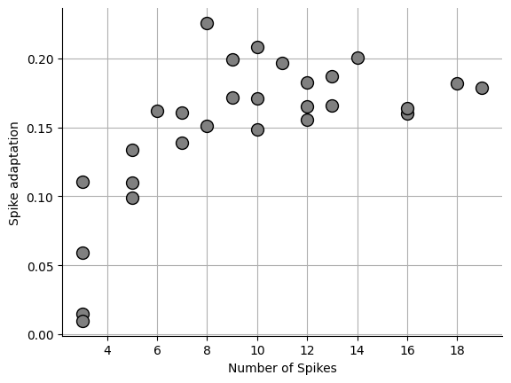
This is the simplest method. The coefficient of variation (CV) is the standard deviation of IEIs divided by the mean IEI. The CV measures the dispersion of the data.

sa = []
npeaks = []
for acq in exp_dict.values():
    p = acq["peaks"]
    acq["cv"] = np.nan
    if len(p) > 1:
        iei = np.diff(p)
        spike_adapt = np.std(iei) / np.mean(iei)
        sa.append(spike_adapt)
        npeaks.append(len(p))
        acq["cv"] = spike_adapt
fig, ax = plt.subplots()
print(np.mean(sa))
ax.set_xlabel("Number of Spikes")
ax.set_ylabel("Spike adaptation")
ax.grid(which="both")
ax.spines["top"].set_visible(False)
ax.spines["right"].set_visible(False)
_ = ax.plot(npeaks, sa, "o", markersize=10, markerfacecolor="grey", markeredgecolor="black")

0.15048103024136505

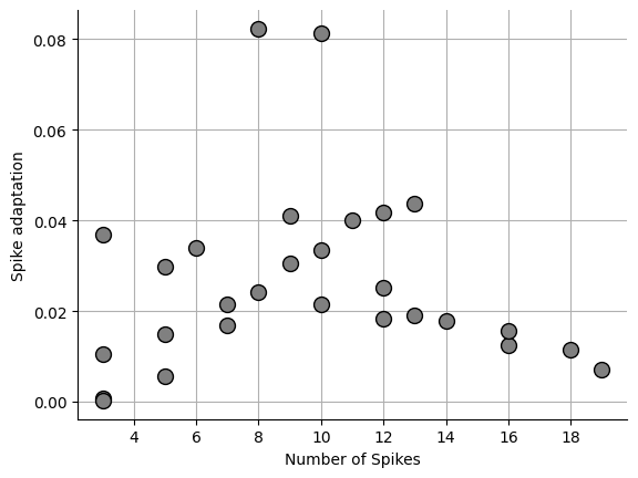
Local variation¶

Local variation is from Shinomoto et al., 2009 Shinomoto et al., 2009. One problem with the CV is that vastly different spike patterns can result in the same CV. Shinomoto developed an equation that get around that issue.

sa = []
npeaks = []
for acq in exp_dict.values():
    p = acq["peaks"]
    acq["local_sfa"] = np.nan
    if len(p) > 2:
        iei = np.diff(p)
        isi_shift = iei[1:]
        isi_cut = iei[:-1]
        n_minus_1 = len(isi_cut)
        local_var = (
            np.sum((3 * (isi_cut - isi_shift) ** 2) / (isi_cut + isi_shift) ** 2)
            / n_minus_1
        )
        sa.append(local_var)
        acq["loca_sfa"] = local_var
        npeaks.append(len(p))
fig, ax = plt.subplots()
print(np.mean(sa))
ax.set_xlabel("Number of Spikes")
ax.set_ylabel("Spike adaptation")
ax.grid(which="both")
ax.spines["top"].set_visible(False)
ax.spines["right"].set_visible(False)
_ = ax.plot(npeaks, sa, "o", markersize=10, markerfacecolor="grey", markeredgecolor="black")

0.02637187438528412

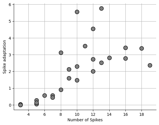
Revised local variation¶

Revised local variation is from Shinomoto et al., 2009 Shinomoto et al., 2009. One problem with the CV is that vastly different spike patterns can result in the same CV. Shinomoto originally developed the local variation equation to fix this issue, however they later adjusted the equation to account for the refactory period of the neuron in being analyzed.

sa = []
npeaks = []

# Generic refactory periond of 2 ms will work.
R = 2
for acq in exp_dict.values():
    p = acq["peaks"]
    acq["rlocal_sfa"] = np.nan
    if len(p) > 2:
        iei = np.diff(p / 10)
        isi_shift = iei[1:]
        isi_cut = iei[:-1]
        isi_add = isi_cut + isi_shift
        left = 1 - ((4 * isi_cut * isi_shift) / isi_add**2)
        right = 1 + ((4 * R) / isi_add)
        var = 3 * np.sum(left * right) * len(isi_shift)
        sa.append(var)
        acq["rlocal_sfa"] = var
        npeaks.append(len(p))
fig, ax = plt.subplots()
print(np.mean(sa))
ax.set_xlabel("Number of Spikes")
ax.set_ylabel("Spike adaptation")
ax.grid(which="both")
ax.spines["top"].set_visible(False)
ax.spines["right"].set_visible(False)
_ = ax.plot(npeaks, sa, "o", markersize=10, markerfacecolor="grey", markeredgecolor="black")

1.966381052048725

Spike threshold¶

Spike threshold is tells you at what voltage a cells spike is elicited. This different from rheobase. Spike threhold is primarly set by the number of sodium channels on the axon hillock. The spike threshold is important because it is a bifurcation point in the function of a neuron. If you want to read more about this I suggest reading “Dynamical systems in neuroscience: the geometry of excitability and bursting” Izhikevich, 2007. A lower spike threshold can show up as a lower rheobase in neurons whose voltage continues to rise during the current injection before a spike occurs. I have seen this occur in cortical pyramidal neurons and spiny projection neurons but not parvalbumin inhibitory neurons.

You can measure spike threshold on any acquisition that has a spike, however usually just the spikes from the rheobase acquisitions are used to calculate the spike threshold. There are several ways to calculate the spike threshold such a the first derivative, second derivative, third derivative, and a max curvature Sekerli et al., 2004. I find the third derivative and method VII to be the most consistent. We will use the third derivative method in this tutorial. The way I typically differentiate signals is by using Numpy’s gradient. Unlike diff, gradient returns an array of the same length as the input signal which makes downstream analysis easier. It has the downside in that if you have small peaks you will get some artifacts in the signal which upsampling can counteract. One problem I found with the third derivative is that the peaks found a usually to late by 1 sample at 10000 Hz so I adjust the spike threshold backwards by 1 sample. I also z-score the derivative since this keeps the peak finding threshold consistent between acquisitions.

First lets look a single acquisition and see how the different derivatives look. One thing we are going to do just for visualization purposes is limit the extent of the x-axis so that we are just looking at the first spike and for a point of reference we are going to use the spike peak. If you look at the third derivative we want to extract the first positive peak. There are some additions that I have found are helpful.

voltages = np.array(exp_dict[rheobase_acq[0]]["array"])
peak = exp_dict[rheobase_acq[0]]["peaks"][0] - pulse_start

# grab the voltages just inside the current pulse
voltages = voltages[pulse_start:pulse_end]
x = np.arange(voltages.size)

# First derivative
dv = np.gradient(voltages)
# Second derivative
ddv = np.gradient(dv)
# Third derivateive
dddv = np.gradient(ddv)

fig, ax = plt.subplots(nrows=2, ncols=2, constrained_layout=True)
ax = ax.flat
for index, j in enumerate([("Voltage (mV)", voltages), ("dV",dv), ("ddV", ddv), ("dddV",dddv)]):
    ax[index].set_title(j[0])
    ax[index].plot(x[1120:1220], j[1][1120:1220])
    ax[index].axvline(peak, color="orange", linewidth=2)
    ax[index].grid(which='both')
    ax[index].spines["top"].set_visible(False)
    ax[index].spines["right"].set_visible(False)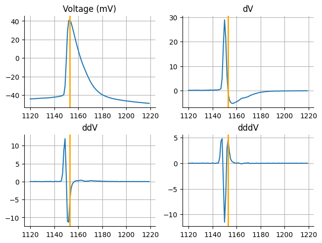

We are going to calculate the spike threshold for every spike in an acquisition that contains spikes. We will use the third derivative method. To do this we will create two functions. One to find a spike threshold for a single spike in a window. The second function will loop through all of the spikes to find the spike threshold using a different start and stop values for each spike.

def find_spk_threshold(voltages: np.array, start: int, end: int):
    dv = np.gradient(voltages)
    ddv = np.gradient(dv)
    dddv = np.gradient(ddv)

    temp = dddv[start:end]
    base = temp.argmin()
    index = base - 1
    val = temp[base] - temp[index]
    while val < 0:
        index -= 1
        base -= 1
        val = temp[base] - temp[index]
    thresh_peak = start + index
    return thresh_peak


def find_all_spk_thresholds(voltages, peaks, pulse_start):
    output = np.zeros(len(peaks), dtype=int)
    start_index = pulse_start
    for index in range(len(peaks)):
        if index < (len(peaks) - 1):
            end_index = peaks[index]
        else:
            end_index = pulse_end
        output[index] = find_spk_threshold(voltages, start_index, end_index)
        start_index = peaks[index]
    return output


for acq in exp_dict.values():
    voltages = np.array(acq["array"])
    peaks = acq["peaks"]
    if len(peaks) > 0:
        output = find_all_spk_thresholds(voltages, peaks, pulse_start)
        acq["threshold_index"] = output
    else:
        acq["threshold_index"] = None

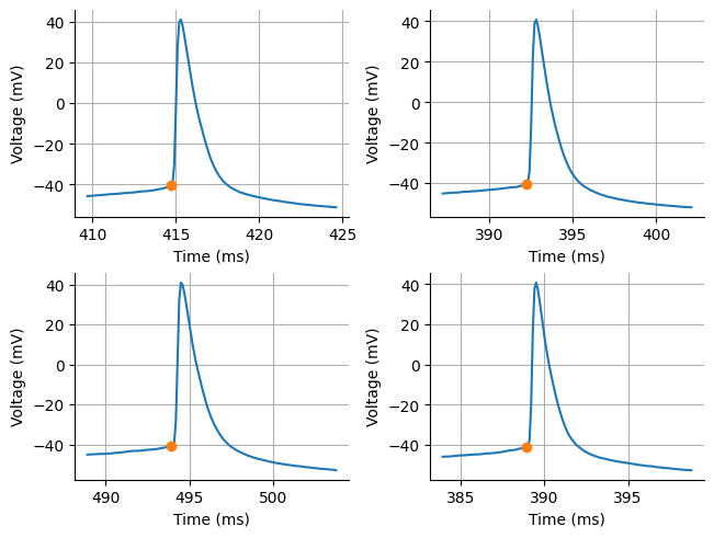
To calculate the spike threshold we are only going to get the spike threshold for the first spike of each rheobase acquisition. This is pretty common practice. Let’s inspect the output. While it may look like the spike threshold is climbing up the spike a little bit, it is important to remember what a failed spike looks like. There is often a hump suggesting there is a small and rapid climb in voltage before a spike can occur even if the spike does not occur. We are trying to find that bifurcation point. Unfortunately, I did not include an acquisition with a failed spike to show the difference.

figures = []

spike_threshold_x = []
spike_threshold_y = []
for i in rheobase_acq:
    index = exp_dict[i]["threshold_index"][0]
    spike_threshold_y.append(exp_dict[i]["array"][index])
    spike_threshold_x.append(index)

temp = {str(i): exp_dict[i]["array"] for i in rheobase_acq}
x = np.arange(len(temp[str(rheobase_acq[0])])) / 10
fig, ax = plt.subplots(nrows=2, ncols=2, constrained_layout=True)
ax = ax.flat
for sx, sy, acq_num, a in zip(spike_threshold_x, spike_threshold_y, rheobase_acq, ax):
    a.set_xlabel("Time (ms)")
    a.set_ylabel("Voltage (mV)")
    a.plot(x[sx-50:sx+100], exp_dict[acq_num]["array"][sx-50:sx+100])
    a.plot(sx/10, sy, "o")
    a.grid(which="both")
    a.spines["top"].set_visible(False)
    a.spines["right"].set_visible(False)

print(f"Spike threshold: {np.mean(spike_threshold_y):.3f} mV")

Spike threshold: -40.635 mV

Spike half-width and width¶

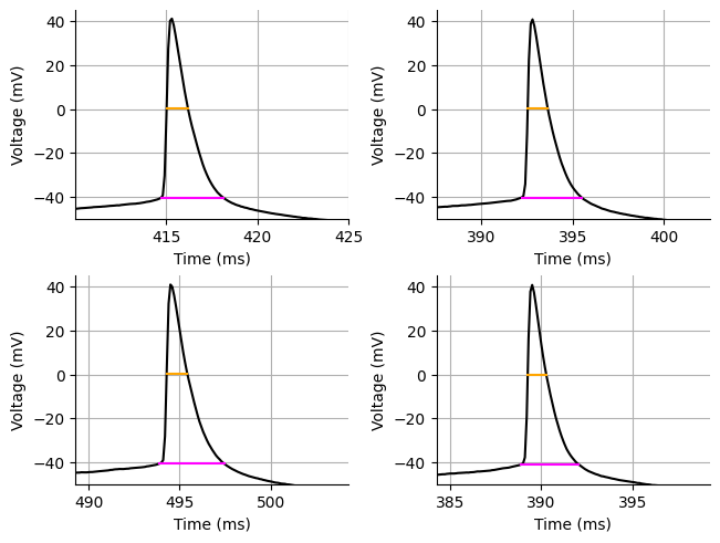
The next waveform feature that we can measure is the spike (half) width. Half width is important because it can help you determine if there is broadening or shortening of the waveform. Broadening of the waveform can be due to inactivation of the voltage-gated potassium channels, slower-inactivating sodium channels or even decreased activation of voltage-gated calcium channels. Wavefrom broadening increases synaptic output by increasing release probability by increasing the time calcium is in the presynapse Zbili & Debanne, 2019. This is where the voltage crosses half way between the spike threshold and peak. One important caveat of measuring spike width as the half-way point is that if your spike threshold or peak is changed then your half-width will likely be different.

We will also measure the full spike width defined as the length of time it takes to go from spike threshold to spike threshold for a single spike. From this we can pull the depolarization time and repolarization time. It is easier to see that the spike is asymmetric with the depolarization being faster than the repolarization.

def find_spk_width(voltages: np.array, start: int, end: int):
    start = int(start)
    end = int(end)
    volts = np.asarray(voltages[start:end])
    xvals = np.linspace(start, end, num=int((end - start) * 10))
    x = np.linspace(start, end, num=int(end - start))
    volts = np.interp(xvals, x, volts)
    spike_threshold = voltages[start]
    masked_array = volts.copy()
    mask = np.array(volts > spike_threshold)
    peak_x = np.argmax(volts)
    masked_array[~mask] = spike_threshold
    hw = signal.peak_widths(masked_array, [peak_x], rel_height=0.5)
    fw = signal.peak_widths(masked_array, [peak_x], rel_height=1)
    return (
        hw[2][0] / 10 + start,
        hw[3][0] / 10 + start,
        hw[1][0],
        fw[2][0] / 10 + start,
        fw[3][0] / 10 + start,
        fw[1][0],
    )


def find_all_spk_widths(voltages, spike_thresholds, pulse_end):
    width_keys = ["hw_left", "hw_right", "hw_y", "fw_left", "fw_right", "fw_y"]
    width = {key: np.zeros(len(peaks)) for key in width_keys}
    for index in range(len(peaks)):
        if index < (len(peaks) - 1):
            end = spike_thresholds[index + 1]
        else:
            # Adding 2000 samples (or 2 ms) to the end helps with spikes that occur just before the end of the acquisition
            if (pulse_end - spike_thresholds[index]) < 2000:
                end = spike_thresholds[index] + 2000
            else:
                end = pulse_end
        output = find_spk_width(
            voltages,
            spike_thresholds[index],
            end,
        )
        for key, value in zip(width_keys, output):
            width[key][index] = value
    return width

spike_width_x = []
spike_width_y = []
for acq in exp_dict.values():
    voltages = acq["array"]
    spk_thresholds = acq["threshold_index"]
    peaks = acq["peaks"]
    if len(peaks) > 0:
        hws = find_all_spk_widths(voltages, spk_thresholds, pulse_end)
        acq.update(hws)
    else:
        width_keys = ["hw_left", "hw_right", "hw_y", "fw_left", "fw_right", "fw_y"]
        width = {key: None for key in width_keys}
        acq.update(width)

To calculate the spike width we are only going to get the spike width for the first spike of each rheobase acquisition. This is pretty common practice. We can also inspect the spike width measurements to make sure they are correct.

figures = []
hw = []
fw = []
fig, ax = plt.subplots(nrows=2, ncols=2, constrained_layout=True)
ax = ax.flat
for acq_num, a in zip(rheobase_acq, ax):
    acq = exp_dict[acq_num]
    sx = [acq["hw_left"][0], acq["hw_right"][0]]
    sy = acq["hw_y"][0]
    sy = [sy, sy]
    hw.append((sx[1] - sx[0]) / 10)
    array = exp_dict[acq_num]["array"]

    a.set_xlabel("Time (ms)")
    a.set_ylabel("Voltage (mV)")
    a.grid(which="both")
    a.spines["top"].set_visible(False)
    a.spines["right"].set_visible(False)
    a.plot(x, array, color="black")
    a.set_xlim(sx[0]/10-5, sx[0]/10+10)
    a.set_ylim(-50,45)
    a.plot(np.array(sx)/10, sy, color="orange")

    sx = [acq["fw_left"][0], acq["fw_right"][0]]
    sy = acq["fw_y"][0]
    sy = [sy, sy]
    fw.append((sx[1] - sx[0]) / 10)
    a.plot(np.array(sx)/10, sy, color="magenta")

print(f"Spike half-width: {np.mean(hw):.3f} ms")
print(f"Spike width: {np.mean(fw):.3f} ms")
# show(gridplot([figures[:2], figures[2:]]))

Spike half-width: 1.109 ms
Spike width: 3.362 ms

Spike Area Under the Curve (AUC)¶

Spike AUC is similar to spike width except that it is the sum of the interaction between spike threshold, peak spike voltage and the spike width. The AUC can be calculated by integrating the spike from the spike threshold to spike threshold. Since we have evenly spaced samples we can use a simple integrating function Numpy’s trapezoid. To improve the quality of the AUC measure we will upsample by 10x. This is probably not need but it is fast and adds very little code.

def find_spk_auc(voltages: np.array, start: int, end: int):
    volts = np.asarray(voltages[int(start) : int(end)])
    spike_threshold = voltages[start]
    x = np.arange(len(volts))
    xvals = np.linspace(x[0], x[-1], num=x.size * 10)
    yinterp = np.interp(xvals, x, volts)
    peak = np.argmax(yinterp)
    indices = np.where(yinterp > spike_threshold)[0]
    splits = np.where(np.diff(indices) > 1)[0]
    if len(splits) > 0:
        indices = indices[: splits[0]]
    yinterp = yinterp - yinterp[indices[0]]
    auc = (
        np.trapezoid(yinterp[indices[:-1]], dx=x[1] / 10 - x[0] / 10),
        np.trapezoid(yinterp[indices[0] : peak + 1], dx=x[1] / 10 - x[0] / 10),
        np.trapezoid(yinterp[peak : indices[-1] + 1], dx=x[1] / 10 - x[0] / 10),
    )
    return auc


def find_all_spk_auc(voltages, spike_thresholds, pulse_end):
    auc_keys = ["auc", "auc_left", "auc_right"]
    auc = {key: np.zeros(len(spike_thresholds)) for key in auc_keys}
    for index in range(len(spike_thresholds)):
        if index < (len(spike_thresholds) - 1):
            end = spike_thresholds[index + 1]
        else:
            # Adding 2000 samples (or 2 ms) to the end helps with spikes that occur just before the end of the acquisition
            if (pulse_end - spike_thresholds[index]) < 2000:
                end = spike_thresholds[index] + 2000
            else:
                end = pulse_end
        output = find_spk_auc(
            voltages,
            spike_thresholds[index],
            end,
        )
        for key, value in zip(auc_keys, output):
            auc[key][index] = value
    return auc

spike_width_x = []
spike_width_y = []
for acq in exp_dict.values():
    voltages = acq["array"]
    spk_thresholds = acq["threshold_index"]
    peaks = acq["peaks"]
    if len(peaks) > 0:
        auc = find_all_spk_auc(voltages, spk_thresholds, pulse_end)
        acq.update(auc)
    else:
        auc_keys = ["auc", "auc_left", "auc_right"]
        auc = {key: None for key in auc_keys}
        acq.update(auc)

auc = []
auc_left = []
auc_right = []
for i in rheobase_acq:
    auc.append(exp_dict[i]["auc"][0])
    auc_left.append(exp_dict[i]["auc_left"][0])
    auc_right.append(exp_dict[i]["auc_right"][0])
print(f"AUC: {np.mean(auc):.3f}")
print(f"Left AUC: {np.mean(auc_left):.3f}")
print(f"Right AUC: {np.mean(auc_right):.3f}")

AUC: 1017.390
Left AUC: 207.321
Right AUC: 810.072

Spike afterhyperpolarization (AHP)¶

The spike afterhyperpolarization (AHP) is the refactory period, the period where a neuron cannot fire another action potential. The AHP is defined as when the membrane voltage drops below the resting membrane potential of a neuron. However, when injecting current in slices or cell culture, you will rarely see the AHP drop below the resting membrane potential or the potential where the cell is being held instead I have seen the AHP defined as when the spike drops below the spike threshold. The are a a couple ways that you could analyze the AHP. One way is setting a cutoff after the spike for what part of the AHP you want to analyze and integrate over that period. One thing to consider with this method is that you will likely want to integrate over a percent of the AHP rather than using a strict time cutoff since the AHP will get shorter at higher spike frequencies. This is typically how people calculate the slow and fast components of the AHP. You can also find the peak or most negative component of the AHP and when it occurs. For our analysis we will analyze the voltage of the peak (most negative) AHP.

Measuring the peak AHP¶

def find_all_ahp_peaks(voltages, peaks, pulse_end):
    output = np.zeros(len(peaks), dtype=int)
    for index in range(len(peaks)):
        if index < (len(peaks) - 1):
            t = np.argmin(voltages[peaks[index] : peaks[index + 1]]) + peaks[index]
        else:
            t = np.argmin(voltages[peaks[index] : pulse_end]) + peaks[index]
        output[index] = t
    return {"ahp_index": output}


for acq in exp_dict.values():
    voltages = acq["array"]
    peaks = acq["peaks"]
    if len(peaks) > 0:
        output = find_all_ahp_peaks(voltages, peaks, pulse_end)
        acq.update(output)
    else:
        acq["ahp_index"] = None

spike_ahp_time = []
spike_ahp_volt = []
for i in rheobase_acq:
    index = exp_dict[i]["ahp_index"][0]
    spike_ahp_time.append(index / 10)
    spike_ahp_volt.append(exp_dict[i]["array"][index])
print(f"AHP time: {np.mean(spike_ahp_time):.3f} ms")
print(f"AHP volt: {np.mean(spike_ahp_volt):.3f} mV")

AHP time: 467.275 ms
AHP volt: -56.525 mV

figures = []
fig, ax = plt.subplots(nrows=2, ncols=2, constrained_layout=True)
ax = ax.flat
for acq_num, a in zip(rheobase_acq, ax):
    acq = exp_dict[acq_num]
    sx = acq["ahp_index"][0] / 10
    sy = acq["array"][acq["ahp_index"][0]]
    array = exp_dict[acq_num]["array"]
    a.set_xlabel("Time (ms)")
    a.set_ylabel("Voltage (mV)")
    a.grid(which="both")
    a.spines["right"].set_visible(False)
    a.spines["top"].set_visible(False)
    a.set_xlim(sx-100, sx+200)
    a.set_ylim(-70,45)
    a.plot(x, array, color="black")
    a.plot(sx, sy, markersize=10, color="orange", marker="o")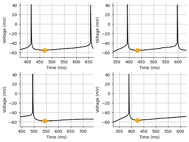

Spike derivative¶

The spike derivative is useful because we can look at the currents underlying the spike itself. While we cannot see the exact Na+, K+ and Ca+ currents we can get an idea of what currents might be altered. To convert a voltage spike to current spike we must multiply the spike derivative by the capacitance of the cell since the current (I) = -C*dV/dt. The current action potential is very similar to the current action potentials that you get when you record spontaneous action potentials is cell-attached voltage-clamp mode. This equation works because a cell is a capacitor due to the lipid membrane. The first peak, or most negative peak primarily consists of Na+ currents where as the second peak likely consists of K+ and Ca+ currents Bean, 2007. One interesting thing to note is the peak current in these spikes (~-2000 pA) is typically around the current you get with unclamped spikes when running a electrical/optical stimulation experiment.

def spk_velocity(dv: np.ndarray, start: int, end: int):
    min_pos = np.argmin(dv[start:end]) + start
    min_val = dv[min_pos]
    max_pos = np.argmax(dv[start:end]) + start
    max_val = dv[max_pos]
    return min_pos, min_val, max_pos, max_val


def find_all_spk_velocities(
    voltages: np.ndarray,
    spike_thresholds: np.ndarray,
    pulse_end: int,
    end_offset: int = 2000,
):
    keys = ["min_velocity_pos", "min_velocity", "max_velocity_pos", "max_velocity"]
    velocity_measures = {key: np.zeros(spike_thresholds.size) for key in keys}
    dv = -1 * np.gradient(voltages)
    for index in range(spike_thresholds.size):
        if index < (len(spike_thresholds) - 1):
            end = spike_thresholds[index + 1]
        else:
            # Adding end_offset samples (or 2 ms) to the end helps with spikes that occur just before the end of the acquisition
            if (pulse_end - spike_thresholds[index]) < end_offset:
                end = spike_thresholds[index] + end_offset
            else:
                end = pulse_end
        output = spk_velocity(dv=dv, start=spike_thresholds[index], end=end)
        for key, value in zip(keys, output):
            velocity_measures[key][index] = value
    return velocity_measures

for acq in exp_dict.values():
    voltages = acq["array"]
    peaks = acq["peaks"]
    if len(peaks) > 0:
        spkt = acq["threshold_index"]
        temp = find_all_spk_velocities(voltages, spkt, pulse_end)
        acq["velocity"] = temp
    else:
        acq["velocity"] = None

first_spikes = []
offset = int(1 * 10)
for acq in rheobase_acq:
    array = exp_dict[acq]["array"]
    index = exp_dict[acq]["threshold_index"][0]
    start = index - offset
    if exp_dict[acq]["threshold_index"].shape[0] > 1:
        end = int(exp_dict[acq]["threshold_index"][1])
    else:
        peak_x = exp_dict[acq]["peaks"][0]
        thresh = exp_dict[acq]["array"][index]
        ind = np.where(array[peak_x:] < thresh)[0] + peak_x
        end = min(ind[-1], pulse_end)
    first_spikes.append(array[start:end])

min_len = min([len(i) for i in first_spikes])
first_spikes = [i[:min_len] for i in first_spikes]
derivative = [np.gradient(i) * -85 for i in first_spikes]
peak_na = np.mean([min(i) for i in derivative])
peak_k_ca = np.mean([max(i) for i in derivative])
print(f"Peak Na+: {peak_na} pA; Peak K+/Ca2+: {peak_k_ca} pA")

Peak Na+: -2463.1133098886303 pA; Peak K+/Ca2+: 477.5992611348708 pA

fig, ax = plt.subplots(ncols=3, figsize=(8,3), constrained_layout=True)
ax[0].set_ylabel("mV")
ax[1].set_ylabel("pA")
ax[1].set_xlim(0,40)
ax[2].set_ylabel("pA")
ax[2].set_xlabel("mV")
for i in ax:
    i.grid(which="both")
    i.spines["right"].set_visible(False)
    i.spines["top"].set_visible(False)
for i, j in zip(first_spikes, derivative):
    x = np.arange(len(i))
    ax[0].plot(x, i, color="black", linewidth=1, alpha=0.5)
    ax[1].plot(x, j, color="black", linewidth=1, alpha=0.5)
    ax[2].plot(i, -j, color="black", linewidth=1, alpha=0.5)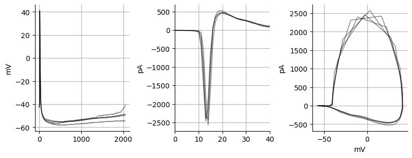

Membrane time constant¶

The membrane time constant is the decay tau of a the exponential decay that the membrane undergoes during negative pulse injects. It gives you an idea of how membrane capacitance and resistance interact. The membrane time constant equation is: $\tau=rc$ . We have to remember that the membrane is a resistor and capacitor in parallel which means when we inject a current it will take time for the membrane to reach a steady state voltage. One factor to consider when measuring the membrane time constant is that you have to choose how to define the amplitude. Do you choose the minimum voltage which could be influenced by HCN channels causing voltage sag or do you choose the delta V that we measured earlier? There are two way you can find the time constant. The first is you can find the time is takes for for the voltage go below 1/3 of the delta V amplitude. Alternatively you can curve fit the voltage trace to an exponential decay. We will not curve fit here because I have found it to be very tricky to curve fit. The main reason is where you choose the start and end effects the quality of the curve fit. Some neurons have voltage sag which means those neurons do not act as a pure RC circuits. Some neurons have a very square shaped voltage response which really throws off the curve fit.

taus1 = []
taus2 = []
pulse_amps = []
for acq in exp_dict.values():
    acq["mem_tau_est1"] = np.nan
    acq["mem_tau_est2"] = np.nan
    if acq["pulse_amp"] < 0:
        voltages = acq["array"] - acq["baseline_v"]
        threshold1 = voltages.min() * 0.33
        threshold2 = acq["delta_v"] * 0.33
        min_val = voltages.argmin() + pulse_start
        indices = np.where(voltages[pulse_start:min_val] < threshold1)[0][0]
        acq["mem_tau_est1"] = indices / 10
        taus1.append(indices / 10)
        indices = np.where(voltages[pulse_start:min_val] < threshold2)[0][0]
        acq["mem_tau_est2"] = indices / 10
        taus2.append(indices / 10)
print(f"Membrane time constant (min value): {np.mean(taus1):.3f} ms")
print(f"Membrane time constant (delta V): {np.mean(taus2):.3f} ms")

Membrane time constant (min value): 7.637 ms
Membrane time constant (delta V): 5.719 ms

Rebound spikes¶

Rebound spikes typically occur after a hyperpolarizing pulse. Dopaminergic cells typically have a rebound spike. I have not seen any analyses of the rebound spike(s), however this is feature that your cell could have and you could note the presence or number of the rebound spike(s).

p = "https://cdn.jsdelivr.net/gh/LarsHenrikNelson/PatchClampHandbook/data/rebound_spike/1.json"
with urllib.request.urlopen(p) as url:
    file = json.load(url)
array = file["array"]
fig, ax = plt.subplots()
ax.plot(np.arange(len(array)), array, color="black")
ax.grid(which="both")
ax.spines["top"].set_visible(False)
ax.spines["right"].set_visible(False)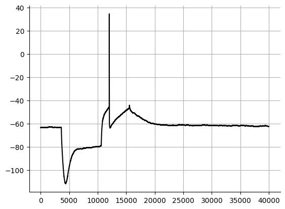

Exporting our data¶

Lastly, we will export our data to a spreadsheet. This part of the analysis is to familiarize you with the dataframe tools and methods (using Pandas), and data export (csv) in Python. I am choosing CSV export over Excel export because CSV is easier to work with downstream. This will enable you to use the notebook as a template for a semiautomated analysis if you want. Additionally the analysis we used here is part of the next section in the current clamp chapter.

Export the spike parameters¶

We will export the spike parameters and the general parameters separately. The spike parameters will be useful

output = defaultdict(list)
for key, i in exp_dict.items():
    if i["voltages"].size > 0:
        output["Threshold (mV)"].extend(i["array"][i["threshold_index"]])
        output["Threshold (ms)"].extend(i["threshold_index"] / 10)
        output["HW (ms)"].extend((i["hw_right"] - i["hw_left"]) / 10)
        output["HW Left (ms)"].extend(i["hw_left"] / 10)
        output["HW Right (ms)"].extend(i["hw_right"] / 10)
        output["HW (mV)"].extend(i["hw_y"])
        output["Spike (mV)"].extend(i["voltages"])
        output["Spike (ms)"].extend(i["peaks"] / 10)
        output["AHP (mV)"].extend(i["array"][i["ahp_index"]])
        output["AHP (ms)"].extend(i["ahp_index"] / 10)
        output["FW (ms)"].extend((i["fw_right"] - i["fw_left"]) / 10)
        output["FW Left (ms)"].extend(i["fw_left"] / 10)
        output["FW Right (ms)"].extend(i["fw_right"] / 10)
        output["Depol time (ms)"].extend((i["peaks"] - i["fw_left"]) / 10)
        output["Repol time (ms)"].extend((i["fw_right"] - i["peaks"]) / 10)
        output["AUC"].extend(i["auc"])
        output["AUC Left"].extend(i["auc_left"])
        output["AUC Right"].extend(i["auc_right"])
        output["Min Velocity"].extend(i["velocity"]["min_velocity"])
        output["Max Velocity"].extend(i["velocity"]["max_velocity"])
        output["Min Velocity (ms)"].extend(i["velocity"]["min_velocity_pos"] / 10)
        output["Max Velocity (ms)"].extend(i["velocity"]["max_velocity_pos"] / 10)
        output["Spike Number"].extend(np.arange(len(i["voltages"])) + 1)
        output["pulse_amp"].extend([i["pulse_amp"]] * len(i["voltages"]))
        output["Acq Number"].extend([key] * len(i["voltages"]))
spike_output = pd.DataFrame(output)
spike_output.to_csv("spike_data.csv", index=False)

Export the acquisition parameters¶

We will grab the acquisition parameters and we will also need to grab the first spike from each acquisition of the spike output data.

output = defaultdict(list)
for key, i in exp_dict.items():
    output["Acq Number"].append(key)
    output["Sag (ms)"].append(i["Sag (ms)"])
    output["Sag (mV)"].append(i["Sag (mV)"])
    output["Delta V (mV)"].append(i["delta_v"])
    output["rheobase"].append(i["rheobase"])
    output["AI SFA"].append(i["ai_sfa"])
    output["Local SFA"].append(i["local_sfa"])
    output["rLocal SFA"].append(i["rlocal_sfa"])
    output["cv"].append(i["cv"])
    output["Spk Freq (Hz)"].append(i["hertz"])
    output["Spk IEI (ms)"].append(
        np.mean(np.diff(i["peaks"]) / 10) if len(i["peaks"]) > 1 else np.nan
    )
    output["Mem Tau 1 (ms)"].append(i["mem_tau_est1"])
    output["Mem Tau 2 (ms)"].append(i["mem_tau_est2"])
    output["Baseline (mV)"].append(i["baseline_v"])
acquisition_output = pd.DataFrame(output)

first_spike_data = spike_output[spike_output["Spike Number"] == 1]
acquisition_output = pd.merge(
    first_spike_data, acquisition_output, on="Acq Number", how="right"
)
acquisition_output.to_csv("acquisition_data.csv", index=False)

That is it for section one of current clamp analysis.

References¶

Ferguson, K. A., & Cardin, J. A. (2020). Mechanisms underlying gain modulation in the cortex. Nat Rev Neurosci, 21(2), 80–92. 10.1038/s41583-019-0253-y
Shinomoto, S., Kim, H., Shimokawa, T., Matsuno, N., Funahashi, S., Shima, K., Fujita, I., Tamura, H., Doi, T., Kawano, K., Inaba, N., Fukushima, K., Kurkin, S., Kurata, K., Taira, M., Tsutsui, K.-I., Komatsu, H., Ogawa, T., Koida, K., … Toyama, K. (2009). Relating Neuronal Firing Patterns to Functional Differentiation of Cerebral Cortex. PLoS Comput Biol, 5(7), e1000433. 10.1371/journal.pcbi.1000433
Izhikevich, E. M. (2007). Dynamical systems in neuroscience: the geometry of excitability and bursting. MIT Press.
Sekerli, M., DelNegro, C. A., Lee, R. H., & Butera, R. J. (2004). Estimating Action Potential Thresholds From Neuronal Time-Series: New Metrics and Evaluation of Methodologies. IEEE Trans. Biomed. Eng., 51(9), 1665–1672. 10.1109/TBME.2004.827531
Zbili, M., & Debanne, D. (2019). Past and Future of Analog-Digital Modulation of Synaptic Transmission. Digital Transmission.
Bean, B. P. (2007). The action potential in mammalian central neurons. Nature Reviews Neuroscience, 8, 451–465.

Chapters

Current clamp

Chapters

Current clamp: Part 2