Understanding data

One of the biggest issues with data analysis in the biological sciences is that many scientists do not understand the fundamentals of their own data. The reason this problem exists is the most common plotting and statistics program used by scientists is not flexible enough to really explore data in a meaningful way. Additionally, there are usually no courses on data analysis that focus on practicality and intuition. Courses typically get bogged down in mathematics which I do not think you need to start to understand your data. Here, we are going to cover how to describe basic data types and how to visualize data so we can see what our data is like. There are several data types you will encounter, namely continuous, count and categorical. Describing the data type your data is relies on understand how your data is generated and should be done before visualizing and running analysis/statistics on your data.

Contiuous data¶

Continuous values can take on any infinity small decimal point between two real values compared to discrete values which are limited to specific steps (see Wikipedia). Membrane resistance, rheobase, time in an area, etc are all continuous data. Continuous data has two main features; bounds and shape. Sometimes we have a theoretically continuous variable that ends up more discrete due to how we collect the data. For example, rheobase is discretized by using a limited number of current injection steps. Discretized values are more likely to be repeated in a dataset than continuous values. However, we usually treat values that have been discretized by data collection methods as continuous.

Feature of continuous data¶

Bounds¶

A lot of scientific data has bounds on the possible values that the data can be. Typical bounds can be from ($-\infty$, $\infty$), (0, $-\infty$) or (0,1). For example membrane resistance cannot be less than zero but can go to infinity. Spike threshold could technically be negative or positive even though it is unlikely to be positive, so it is unbounded theoretically but bounded biologically. Time values are continuous but become discrete to digitization. Some values become artificially bounded by our ability to detect. mEPSC amplitude cannot be below zero pA however we often set an analysis cutoff above zero pA which truncates the data. Sometimes truncation can cause problems for analysis if the truncation is too sharp in which case you may need to redesign your experiment.

Location¶

Location can be thought of as an additive parameter that shifts the data along the x-axis without changing is shape. To shift the location of your data just added or subtract a constant value. The mean and median are considered location parameters.

Scale¶

Scale relates to the range of values you are likely to get from your data and is probably the most important feature of our data. If you multiply, divide or log transform your data, you are changing the scale of your data. The standard deviation is an example of scale. The larger the standard deviation is the larger the values you have. Quantiles/percentiles are another common value that can discribe the scale of your data. Also note that the standard error of the mean (SEM) is not a scale measure but a precision measure. Lastly, most statistic tests we use assume that the scale is the same between the groups. When the scale is not the same between our groups we cannot use most basic statistical test unless we can transform our data so that the scale is the same.

Shape¶

The shape is how wide or narrow (kurtosis), skewed right or left (skew) your data is. It will change the central tendency (most common value) of the distribution but not in the way location does. Shape is a not related to shifting your data. The shape of our data can be seen by plotting our data. Technically, the mathematical definition of shape depends on the underlying distribution however, we can simply a discription of shape using quantiles. If you have some form of categorical data your data does not have shape and visualization will be much different.

Skew¶

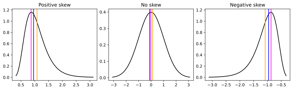
Skew is whether the data tends have more low values than high values or vice versa if your were to split your data by the mean. The shape and scale of a distribution often interact to change a distribution’s skew. Skew can be measured by comparing the distance between 0.75 quantile and median, and the 0.25 quantile and the median or by using the Scipy function skew which uses a moments formula. It is also important to note that skewness measures often fail for multimodal distributions. A common method to measure the skew using the mean and median fails for multimodal distribution.

Kurtosis¶

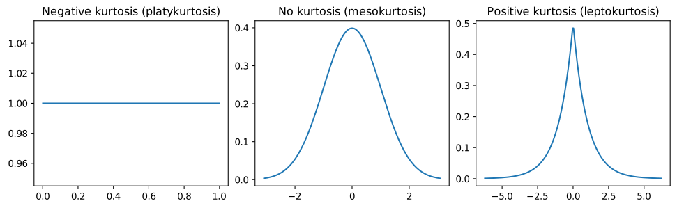
Kurtosis is the tailedness of your data. Long tails increase the chance of getting extreme values. Sometimes we call these outliers. Shape and scale often interact to change a distribution’s kurtosis. Kurtosis can be measured using the Scipy function kurtosis.

Plotting continuous data¶

The most common ways to plot data are to use a error bars plus measure of centrality, box plots, histogram or KDE (note: violin plot is just a KDE). All these methods are non-parametric in that they technically do not have any parameters other than your data to create a distribution. Each method has benefits and draw backs. Error bars plus measure of centrality are the most common but least informative since they usually do no convey information about the shape of the data. Errors bars can show the SEM (not very informative), standard deviation (better), confidence intervals (bootstrapped ared the best) and precentiles (will show the shape of the data). Box plots can convey information about the shape of the data but need more data points than error bars. Box plots show the median, sometimes the mean, the 0.25 and 0.75 quantile and 1.5 times the interquartile range. Histograms are good for larger amounts of data but can be biased by bin width (0-1, 1-2, etc.). KDE needs larger amounts of data but have the least amount of bias. Note that you can turn histograms and KDEs onto their side for typical categorical data.

How to create a box plot¶

A box plot consists of a box that goes from the 0.25 quantile to the 0.75 quantile. There is a line in the middle that is the 0.5 quantile or median. There are whiskers that can be plotted one of two ways. One way is to use the interquartile range (IQR) as is or you can calculate use the minimum point that is closest to the IQR which is useful if the IQR goes beyond any values in your data. The IQR is the difference between 0.75 and 0.25 quantiles times 1.5. Then you add that to the 0.75 quantile or subtract that from the 0.25 quantile.

How to Create a Histogram¶

To create a histogram in Python the easiest way is to use Numpy’s histogram. For this example we will use 50 bins, however Numpy has a pretty good algorithm for automatically selecting bins. One setting we will use is the density equals true. This will ensure that each bin shows the likelihood so that is matches with the KDE. If you just want to plot a histogram in other popular plotting packags such as Matplotlib or Seaborn, they have modules where you can just put in your data.

How to Create a Kernel Density Estimate (KDE)¶

To create a KDE in Python we are going to use Scipy’s gaussian_kde. There are other implementations of KDEs such Scikit Learn and KDEpy.

KDE stands for Kernel Density Estimate. KDE is a non-parametric density function. There is no predefine function to create the PDF from your data, you create a unique one from your data. The aim of the KDE is not to represent the density function of your data exactly as it is, like a histogram but, to represent it as if you had an infinitely large sample size. KDEs can represent your data as it is by setting a feature called the bandwidth. The only real subjective feature of a KDE is how much to “smooth” your probability distribution that the KDE outputs.

The KDE works by essiantially putting a gaussian distribution (or other distribution) around each point of data and then sums them up. Depending on how smooth we want the distribution we can increase or decrease the bandwidth. For the gaussian distribution the bandwidth is related to the standard deviation. The larger the bandwidth the smoother the KDE and vice versa. There are some algorithms to precompute the bandwidth called Silvermans, Scotts and Improved Sheather-Jones (ISJ) if you don’t want to compute the bandwidth yourself however, Scipy does not provide the ISJ algorithm. There are also different ways to compute the KDE such tree and FFT.

Below we will process all the data.

Examining the data¶

Below are some plots of our data using the plotting methods from above. There are two common transforms that we include and explain more below. Look at the data and see how they change. You will also notice I included some lines in the KDE plot. The magenta line would be considered the mode, or the most common value, the blue line is the median and the orange line is the mean. Look at what happens to the relationship between those lines with the different transforms.

Transforms¶

In the plots above, what did you notice when the data transformed? You may have noticed that the whiskers in the box plot become more symmetrical. You may have noticed that the the mean and median lines in the KDE plot get closer together with the square root and log transform. The mean and median also get closer to the mode. When dealing with non-gaussian continuous data we can transform the data to make it gaussian. Perfect gaussian data should have no difference between the mean, median and mode. Most transforms work only with positively skewed data. To transform negatively skewed data we often have to multiply by negative 1. All transforms rescale the data to get it to be more guassian but, the best transforms have interpertability for inferential statistics. Transforms also allow us to use simple statistical models (OLS) rather than relying on more complex models (GLMs). When modeling data we are usually looking for the simplest model to accurately models our data since simple models are much more interpretable.

Square root transform¶

The square root transform is probably the least “strong” common transform for positive skew data.

Log transform¶

The log transform is by far the most useful transform for positive skew data. The log transform works on data that is bounded by zero and goes to positive infinity. You can use any type of base for the log however, the natural log is probably the most common. The log transform is nice because if you log transform normal data is will just be normally distributed. So you could theoretically just log transform everything since in with real data the the np.mean(x) and np.exp(np.mean(np.log(x))) will almost never be the same but very close.

Negative inverse (or the inverse)¶

Good for strongly positive skewed data and also keeps interpretability of a regression model. We take the negative inverse because this keeps the directionality of the data (large values are large and small values are small). Rheobase and membrane resistance are inversely related so if you want to run a correlation between the two this is a good choice.

Box-cox¶

Box-Cox can only be used on positive data and automatically finds the best power transform for positively or negatively skew data.

Yeo-Johnson¶

Similar to Box-Cox but works with negative data on positively or negatively skew data.

Power transform¶

All the transforms we covered are actually specific instances of a power transform. Power transform is just x**y where y is any number. For example the power transform can be the square x**(1/2) or the cube x**3 Transform for data that includes negative numbers and is similar to the log transform.

Rank transform¶

This is more “exotic” transform in that it you lose a lot of interpetibility since it changes based on what data you put in. It is more common in the machine learning field but works well for extremely kurtotic data and works with extreme skew and multimodal data.

Multimodal data¶

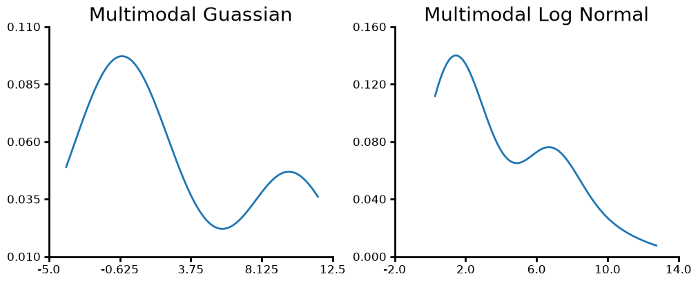
Multimodal data is probably more common than you think. I have seen it several times in “big” data; IEIs for mEPSCs or spikes, mEPSC amplitude at the cell level. For most experiments were we have a summary statistic at the level we run the statistical test on we generally don’t see it. Multimodal data can make our data look non-gaussian when in reality the we have two or more gaussian distributions underlying the full distribution. We can also have multimodal non-gaussian distributions. It is important to remember that you should only look for multimodality when you don’t have some categorical grouping. For example if you have a mix of males and females and see a multimodal distribution that is most likely due to sex differences. If you have a known grouping like sex, genotype, etc., only compare the distribution for each known grouping rather than lumping them all together.

Examples of data principles¶

Next we will work on describing similarities and differences between some data sets.

Scale-Location differences¶

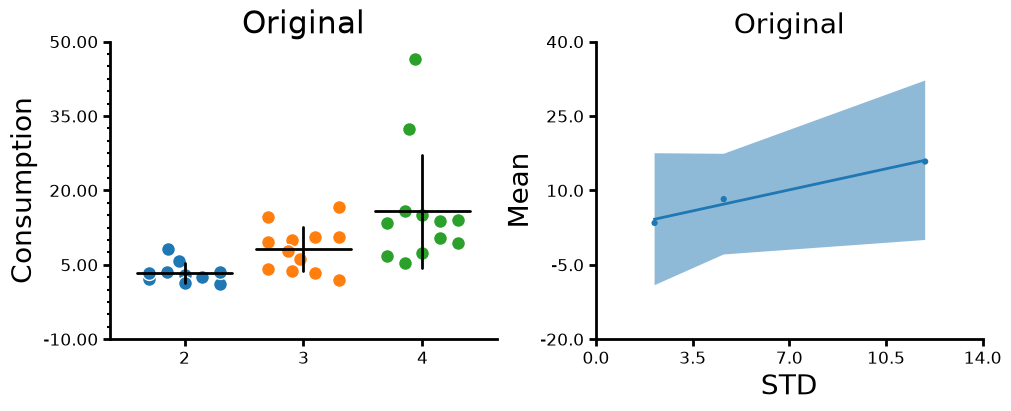
For this dataset on drug consumption you will notice that that the scale, or standard deviation, increases as the mean (location) increases. If scale changes with location then you know you have non-gaussian data. If you do not know whether the mean increases with the scale just a plot a scatter plot of the means vs the standard deviations.

What happens if we log transform the dataset?

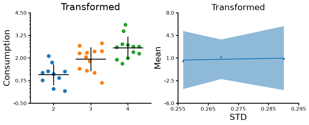
Now you notice that as the mean changes the standard deviation does not change. Also it is important to note that the data is transformed before the we take the mean and standard deviation. To run a statistical test we would do something similar where we would log transform before the test then “back transform” our coefficients and marginal effects. Now that we visualized how log transformation rescales our data let’s look at how the mean change when we log transform the data, get the mean and then back transform the data.

You will notice that the untransformed mean is larger than the transformed mean and that the difference gets larger are the means get larger however, the difference is proportional to the size of the means. So the mean of the data is a consistent just inflated. However, for statistical tests we are also interested in the standard deviation. The standard deviation will still be different between cohorts even transforming and then back transforming like we did with the mean. One caveat with the consumption data is that all the consumption values are coming from a distribution with the same shape and scale since we are dealing with a per subject summary. Total consumption tells you what the end point is not the way you got there. The distribution shape and scale may change with substance consumed, sex, genotype, etc. However, for data like mEPSC IEIs or amplitudes we actually get a different shape/scale per cell.

Count data¶

Count data are things like number of entries into an area, number of spikes or mEPSCs in an acquisition, number of hospital visits, etc. Count data requires specific statistical tests since the data is bounded from zero to infinity and can only be integer numbers.

Categorical data¶

Categorical data is when we assign something to a non-numerical group such male/female or up/down/left/right, true/false, small/medium/large, etc. Categorical data can be ordered or unordered. Unordered would be somethign like male/female and ordered would be like small/medium/large. Sometimes the way we collect data turns a continuous variable into a categorical variable. The Von Frey test uses small wires of increasing gauge to test pain senstivity. Pain is continuous but there are only ~12 wires used for the Von Frey test and in my experience you only need about 4 different wires to find the pain threshold for a cohort of mice.

Levels of data¶

Often in neuroscience, we have data that can be described at different levels. We have acquisitions, cells, slices, mice, litters, trials, etc. These levels can be nested within others. The distribution of your data may change depending on the level your are looking at and whether you have summarized (i.e mean, median) your data. For example if you have a distribution of inter-event intervals (IEIs) the distribution of those events for each cell is likely log normally distributed. If you summarized each cell by taking the mean of the IEI and look at the distribution of the mean IEIs at the cell level they may be normally distributed. Understanding how your data is distributed at each level is important for interpreting your data. For example, the mean of a skewed distribution is going influenced by the number and spread of large values. So if you run statistics on a bunch of means you may actually just be comparing how skewed each of your lower level data is. The question do you really want to test whether you have differences in outliers or rather differences in location of you distribution?

Working with nested data is very challenging especially if your data at the lower level is not normally distributed. You have to rely on heirarchical statistics and using non-normal distributions which making interpreting your data and statistical harder. Additionally, the hierarchical/mixed models have questionable p-values since they tend to over estimate effect sizes due to assumptions they make by using the asymmptotic behavior of distributions (basically what happens when your sample size is assumed to infinitely large). However, summarizing data also present a challenge. You need to decide at what level to summarize your data and what summary statistic is best. It can get even harder when the variable you want to summarize depends on or is correlated with another variable. Summarizing your data will hide this dependence and can give you a bad result. Summarizing data has one big benefit in terms of statistical tests: your summarized data, such as the means of IEIs from a bunch of cells, will often be normally distributed. This is due to something called the central limit theorem where the distribution of sample means (means of each cell’s IEI distribution) will be normal.